Gauss’ law for electrostatics
Read Tipler and Mosca (2004) chapters 21 and 22
(The electric field I and II); Pelcovits and Farkas (2024) chapter 11
(Gauss’s law). See also https://www.youtube.com/watch?v=Zu2gomaDqnM
Gauss’s law
Electric flux
The flux of a vector field is a quantity that reflects how much of the field is passing through an area. The fourth equation on the AP Physics C Electricity & Magnetism equation sheet gives the electric flux: \[\Phi_E = \iint \vec{E} \cdot d\vec{A}.\qquad{(1)}\]
In eq. 1, the notation \(d\vec{A}\)
means \(\hat{n} dA\), where \(\hat{n}\) is the normal to \(dA\), so that the fluxfrom fluxus, from Latin, fluere, “to
flow”
quantifies how much field is flowing through the area,
normal to it. The dot product with the normal means we do not count
stuff passing parallel to the area, which doesn’t really flow through
it. We will see similar fluxes for magnetic fields and current. Flux
also occurs in other fields like heat and mass transfer, nuclear reactor
theory, fluid mechanics, and more.
The \(\iint dA\) notation means we
are doing a double integralYou probably are not yet doing these in your
multivariate calculus class, but you will. Typical applications of
double integrals are to find areas (\(\iint
dA\)), moments of area (\(\iint r^2
dA\)), surface areas, cumulative probabilities under multivariate
pdfs, etc. There are also triple integrals, often used to find volumes
(e.g. \(\iiint dV\)).
over an area. You are used to doing a single integral,
e.g. \(\int dx\). A double integral
could be the integral of an integrand that itself is an integral, such
as \(\int \int dx dy\), perhaps
rewritten as \(\iint dA\) to be less
cumbersome. Sometimes, in the interest of writing quickly, we may write
\(\int dA\), recognizing it as a double
integral because it is with respect to \(dA\).
Integral form of Gauss Law
Gauss’s lawDeveloped some by Joseph-Louis Lagrange in 1773; mainly
by Carl Freidrich Gauss in 1835. See also https://en.wikipedia.org/wiki/Gauss\%27s_law. Gauss’s
law is the first of four Maxwell’s Equations which
describe electromagnetic fields; we’ll get to the other three
later.
relates the electric flux out of an arbitrary closed
contour to the charge enclosed (\(q_{enc}\)) within the countour: \[\begin{aligned}
\oiint \vec{E}\cdot d\vec{A} &= 4\pi k q_{enc} \\
&= \dfrac{1}{\epsilon_0} q_{enc}
\end{aligned}\qquad{(2)}\]
The notation \(\oiint d\vec{A}\) means the flux is taken over a closed contour. The contour can be any conveniently chosen shape so long as it has no holes and doesn’t leak. You could choose to integrate over the surface of a potato shape; more often however, the contour is a well-chosen sphere or cylinder.
In eq. 2, \(q_{enc}\) is the charge enclosed within the contour. The actual distribution of the charge within the contour does not really matter for application of eq. 2.
Gauss’s law is a bit funny in that it doesn’t work directly with
\(\vec{E}\) but rather it is a
statement about the double integral of \(\vec{E}\) over some closed contour. At
first sight, these would seem to leave us worse off by adding all kinds
of confusing advanced math to the stuff we must think about. In
practice, however, we can sneak around the advanced math by
making wise choices of the closed contour we integrate over, turning the
multivariate calculus into a geometry problemIn 6.003 Signals and Systems, MIT EECS Prof Stephen
Senturia used to say “We don’t want to do math! We suck at math! We make
stupid mistakes when we try to do math!” suggesting we should find
clever ways to get around actually doing the math. Compare to Chinese
warrior philosopher Sun Tzu (544-496 BCE), “The supreme art of war is to
subdue the enemy without fighting.” Checkmate.
.
For now, we will start using Gauss’s law without deriving it. Gauss’s law can be developed from Coulomb’s law using some multivariate calculus sleight of hand and the sifting properties of the Dirac delta function, but we will not yet go there because you have yet to get to these in your multivariate calculus class.
Differential form of Gauss’s Law (optional aside)
eq. 2 is the integral form of Gauss’s law; there is also a
differential form: \[\vec{\nabla}\cdot\vec{E}=\dfrac{\rho}{\epsilon_0}.\qquad{(3)}\]
The differential form is often put on t-shirts at fancy engineering
schools but is not in any way testable in AP Physics C
Electricity and MagnetismIt is mentioned here merely for those of you who love
seeing odd math and new math symbols so much that it makes you want to
go out and know what the heck these things mean… You may see this in an
physics (e.g. 8.022) or multivariate calculus (e.g. 18.023) class next
year.
.
While the integral form is useful when symmetry and geometry in the
problem allows us to pick a convenient contour, the differential form is
more usable otherwise. The fancy \(\vec{\nabla}\cdot\vec{E}\) notation means
the divergence of \(\vec{E}\), a multivariate calculus
operation that works kind of like our flux calculation as we shrink our
closed contour to be very tiny. There are several multivariate calculus
theorems that become useful when relating such quantities to path, area,
and volume integrals which they will go over later. The upside-down
triangle\(\vec{\nabla}\) is
typically spoken as “del”
\(\vec{\nabla}\) is a
multivariate differential calculus vector operator given in Cartesian
coordinates by \[\vec{\nabla}=\dfrac{\partial}{\partial x}\hat{i}
+ \dfrac{\partial}{\partial y}\hat{j} + \dfrac{\partial}{\partial
z}\hat{k}.\]
Gauss’s law solution for a point charge
{#fig:gausslawpoint} 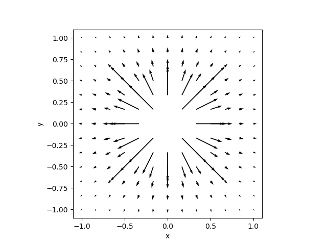
To illustrate the utility of eq. 2 let us first find the
electric field for a point charge \(Q\)
at the origin. We select as a contour a sphere of radius \(r\) centered at the origin.
\[\oiint_{\text{sphere}} \vec{E}\cdot d\vec{a} = 4\pi k Q.\qquad{(4)}\]
Based on symmetry, the \(\vec{E}\) field must point radially everywhere and should only depend on \(r\). Also, the normal to our chosen sphere contour also point radially. These simplify the integral in the left hand side of eq. 4 considerably, allowing us to ditch the dot product and pull \(|\vec{E}|\) out of the integral. \[|\vec{E}| \oiint_\text{sphere} da = 4\pi k Q.\]
The integral over the sphere of \(da\) is just the area of the sphere (\(A=4\pi r^2\)), so that \[\begin{aligned} |\vec{E}| 4\pi r^2 &= 4\pi k Q \\ |\vec{E}| &= \dfrac{kQ}{r^2} \\ \vec{E}(r) &= \dfrac{kQ}{r^2} \hat{r}=\dfrac{1}{4\pi\epsilon_0}\dfrac{Q}{r^2}\hat{r}. \end{aligned}\qquad{(5)}\] which matches what we got from Coulomb’s Law force divided by (test) charge. The final step in eq. 5 recognizes that we used symmetry to conclude the electric field must point radially.
Gauss law solution for an infinite line charge with charge density \(\lambda\)
{#fig:gausslawline} Gauss’s law contour for electric
field from a line charge of charge density \(\lambda \unit{\coulomb\per\meter}\). 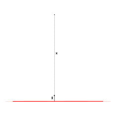
Consider an infinite line charge of charge density \(\lambda\) C m−1 distributed
along its length. Previously, we developed an expression for the
electric field by breaking the line charge into small \(dq\), finding the small contributions \(d\vec{E}\) to the electric field, and
integrating them all. It required trig substitution and got sort of
ugly.
Our approach here using Gauss’s law will be:
Select a contour that exploits symmetry and geometry of the problem. In this problem, we pick a cylinder of radius \(r\) and length \(l\), concentric with the line charge, allowing \(l\) to grow big if we want.
For a well-chosen contour, stuff should pull out of the Gauss’s law integral, changing the multivariate calculus problem to geometry. We will need that the area of a cylinder is \(A=2\pi r l\).
We also note that the cylinder endcaps’ normals \(\hat{n}\) point in the \(\pm z\) direction, while due to symmetry the electric field must point in the \(r\) direction, perpendicuar to \(\hat{n}\). Due to the dot product, the endcaps’ contribution to \(\oiint \cancelto{0}{\vec{E}\cdot d\vec{a}}\) is zero.
Use the charge density to find \(q_{enc}\), i.e. \(q_{enc}=\lambda l\).
Simplify. Have a cup of Earl Grey teaA black tea blend flavored with oil of bergamot (Citrus bergamia), possibly associated with Charles, 2nd Earl Grey; and with fictional Captain Jean-Luc Picard from Star Trek: The Next Generation. Tea of choice of nerds everywhere. See also https://en.wikipedia.org/wiki/Earl_Grey_tea
in the time saved compared to doing the line integral. Tea of choice of nerds everywhere.
\[\begin{aligned} \oiint\vec{E}\cdot d\vec{a} &= 4\pi k q_{enc} \\ |\vec{E}| \iint_\text{cylinder} da &= 4\pi k q_{enc} \\ |\vec{E}| 2\pi r l &= 4\pi k q_{enc} \\ |\vec{E}| 2\cancel{\pi} r \cancel{l} &= 4\cancel{\pi} k \lambda \cancel{l} \\ |\vec{E}| &= 2 k \lambda \dfrac{1}{r} \\ \vec{E}(r) &= 2 k \lambda \dfrac{1}{r} \hat{r}=\dfrac{\lambda}{2\pi\epsilon_0}\dfrac{1}{r}\hat{r}. \end{aligned}\]
Gauss’s law solution for a plane with charge density \(\sigma\)
{#fig:gausslawplane} Gauss’s law contour for electric
field for a plane of charge density \(\sigma
\unit{\coulomb\per\meter\squared}\). 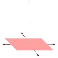
Consider an \(xy\) plane
with charge density \(\sigma\)
C m−2 distributed over its surface. We choose a contour
consisting of a cylinder with long axis along the \(z\) axis, with the plane passing through
its middle. We allow the cylinder radius to be as large as we like. By
symmetry the field must point away from the plane in the \(\pm z\) direction, so that the only
contributions in the Gauss’s law integral are from the endcaps of the
cylinder. Application of Gauss’s law proceeds in a straightforward
manner:
\[\begin{aligned} \oiint\vec{E}\cdot d\vec{a} &= 4\pi k q_{enc} \\ |\vec{E}| 2 \iint_\text{ends} da &= 4\pi k q_{enc} \\ |\vec{E}| 2 \pi r^2 &= 4\pi k q_{enc} \\ |\vec{E}| 2 \cancel{\pi r^2} &= 4\pi k \sigma \cancel{\pi r^2} \\ |\vec{E}| &= 2\pi k \sigma\\ \vec{E}(z) &= \begin{cases} 2\pi k \sigma \hat{z} = \dfrac{\sigma}{2\epsilon_0} \hat{z} & z \geq 0 \\ -2\pi k \sigma \hat{z} = -\dfrac{\sigma}{2\epsilon_0} \hat{z} & z<0 \end{cases} \end{aligned}\]
Gauss’s law solutions for cylinders of radius \(R\)
Thin cylindrical shell with charge density \(\sigma\)
We choose a cylindrical contour of radius \(r\). There are two solutions.
Where \(r<R\), \(q_{enc}=0\) so by inspection \(\vec{E}=0\) for \(r<R\).
Where \(r>R\), the solution
should look just like our line charge solutionIn physics, it is nice to turn a problem into one you
already know how to do.
, with \(\lambda = \sigma 2\pi
R\); but let’s do it out anyway.
\[\begin{aligned} \oiint\vec{E}\cdot d\vec{a} &= 4\pi k q_{enc} \\ |\vec{E}| \iint_\text{cylinder} da &= 4\pi k q_{enc} \\ |\vec{E}| 2\pi r l &= 4\pi k q_{enc} \\ |\vec{E}| 2\pi r l &= 4\pi k \sigma 2\pi R l \\ |\vec{E}| &= 4\pi k \sigma \dfrac{R}{r} \\ \vec{E}(r) &= \begin{cases} 0 & r < R \\ 4\pi k \sigma R \dfrac{1}{r} \hat{r} = \dfrac{\sigma R}{\epsilon_0} \dfrac{1}{r} \hat{r} & r \geq R \end{cases} \end{aligned}\]
Solid cylinder with charge density \(\rho\)
{#fig:gausslawsolidcylinder} Gauss’s law contour for
electric field for a solid cylinder with charge density \(\rho \unit{\coulomb\per\meter\cubed}\).
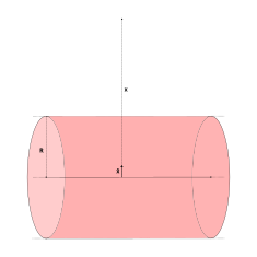
For a solid cylinder of radius \(R\) with charge density \(\rho\) C m−3, the solution for
\(r>R\) should look identical to the
solutions for a line charge (\(\lambda=\pi R^2
\rho\)) or a cylindrical shell (\(\sigma = \frac{R}{2}\rho\)).
\[\begin{aligned} \oiint\vec{E}\cdot d\vec{a} &= 4\pi k q_{enc} \\ |\vec{E}| \iint_\text{cylinder} da &= 4\pi k q_{enc} \\ |\vec{E}| 2\pi r l &= 4\pi k q_{enc} \\ |\vec{E}| 2\pi r l &= 4\pi k \rho \pi R^2 l \\ |\vec{E}| &= 2\pi k \rho \dfrac{R^2}{r} \\ \end{aligned}\]
For \(r<R\), inside the solid cylinder, \[\begin{aligned} \oiint\vec{E}\cdot d\vec{a} &= 4\pi k q_{enc} \\ |\vec{E}| \iint_\text{cylinder} da &= 4\pi k q_{enc} \\ |\vec{E}| 2\pi r l &= 4\pi k q_{enc} \\ |\vec{E}| 2\pi r l &= 4\pi k \rho \pi r^2 l \\ |\vec{E}| &= 2\pi k \rho r \\ \end{aligned}\]
The electric field is \[\vec{E}(r) = \begin{cases} 2\pi k \rho r \hat{r} & r < R \\ 2\pi k \rho R^2 \dfrac{1}{r} \hat{r} & r \geq R \end{cases}\]
Gauss’s law solutions for spheres of radius \(R\)
We remind ourselves that for a sphere of radius \(R\), \(A = 4\pi R^2\) and \(V=\frac{4}{3}\pi R^3\).
Thin spherical shell with charge density \(\sigma\)
{#fig:gausslawsphericalshell} Gauss’s law contour for
electric field for a thin spherical shell with charge density \(\sigma \unit{\coulomb\per\meter\squared}\).
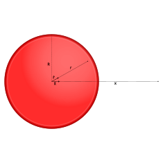
Choose a Gauss’s law contour that is a concentric sphere
of radius \(r\). Where \(r>R\) the solution will look like a
point charge with \(Q=\sigma 4\pi
R^2\). Inside the spherical shell, \(q_{enc}=0\) so by inspection \(\vec{E}=0\) for \(r<R\).
\[\vec{E}(r) = \begin{cases} 0 & r < R \\ \dfrac{4 \pi R^2 \sigma k}{r^2}\hat{r} & r \geq R \end{cases}\]
Solid sphere \(\rho\)
{#fig:gausslawsphere} Gauss’s law contour for
electric field for a solid sphere with charge density \(\rho \unit{\coulomb\per\meter\cubed}\).
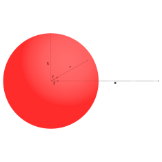
It is left as an exercise for the student to show
that
\[\vec{E}(r) = \begin{cases} \dfrac{4 \pi \rho k}{3} r \hat{r} & r < R \\ \dfrac{4 \pi R^3 \rho k}{3 r^2}\hat{r} & r \geq R \end{cases}\]
See also
MIT 8.02 Walter Lewin video https://www.youtube.com/watch?v=Zu2gomaDqnM
The Mechanical Universe electric field video https://www.youtube.com/watch?v=wq9TjQZDrAA