⊕Read Tipler and Mosca (2004) chapters 21 and 22 (The electric field I and II); Pelcovits and Farkas (2024) chapter 10 (Electrostatics). See also https://www.youtube.com/watch?v=mdulzEfQXDE.

Electric field

Huh? What’s a field? What’s a vector-valued function?

An aside: gravitational field

The magnitude of the gravitational force was given by \[F = \dfrac{G M_1 M_2}{r^2}.\] It is always attractive. Consider the case where we are a tiny mass \(m_2\) compared to a relatively ginormously large \(M_1\) mass nearby. We might like to get our acceleration based on being near the larger mass, and we could get it by dividing the force by our own tiny mass. The magnitude of this acceleration is \(g\)Our friend from AP Physics C Mechanics, \(g=\qty{9.8}{\meter\per\second\squared}\) comes from here. \(G=\qty{6.67e-11}{\meter\cubed\per\kilo\gram\per\second\squared}\), \(M_E=\qty{5.97e24}{\kilo\gram}\) and \(R_E\approx\qty{6.37e6}{\meter}\); \(g=\frac{GM_E}{R_E}\). However, the earth is not perfectly spherical nor is it uniformly dense, leading to local variations in \(g\) that can be mapped with sufficiently sensitive instrumentation. \(g\) is also different on different planets.

: \[g = \dfrac{G M_1}{r^2},\] and the acceleration should point towards the center of the large mass \(M_1\).

Recognizing that the acceleration \(\vec{g}\) is a vector valued function of our position, e.g. \(\vec{g}(\vec{r})\), and also noting the symmetry around a point mass in the \(\theta\) and \(\phi\) directions so that it is only dependent on \(r\): \[\vec{g}(r) = -\dfrac{G M_1}{r^2} \hat{r}.\]

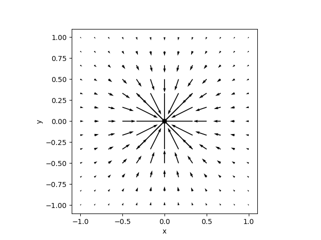
Figure 1: Notional inverse square law gravitational field for a point mass at (0,0). Large vectors near zero have been masked from the quiver plot. — Figure 1: Notional inverse square law gravitational field for a point mass at \((0,0)\). Large vectors near zero have been masked from the quiver plot.

A map of this for some made up silly numbers is shown in fig. ¿fig:marginfigure?, fig. 1. We have visualized a vector field; in this case the gravitational field. The gravitational field tells us, for each point in space, where the resulting acceleration points. If we knew the mass, we could multiply it by the gravitational field to get the gravitational force.

Electric field of a point charge

By analogy with the gravitational field, we can do the same for a point charge, beginning from Coulomb’s law: \[|\vec{F_E}| = \dfrac{k q_1 q_2}{r^2}.\]

Instead of dividing force by mass to get acceleration, we divide force by charge to get the magnitude of what we will call the electric field \(\vec{E}\): \[|\vec{E}| = \dfrac{|\vec{F}_E|}{q_2} = \dfrac{k q_1}{r^2}.\]

The electric field \(\vec{E}\) is a vector field that varies spatially. If we multiply the electric field by a test charge (\(q_{2}\) in this case), we get the electrostatic force acting on that test charge: \[\vec{F}_E = \vec{E} q_{2}.\] ⊕Neither eq. 1 nor eq. 2 appear on your equation sheet for the AP Physics C E&M Exam. The closest things you have are Coulomb’s law and the second equation on the sheet, \(\vec{E}=\frac{\vec{F}_E}{q}\). You are expected to be able to get to the electric field from these parts if you need it.

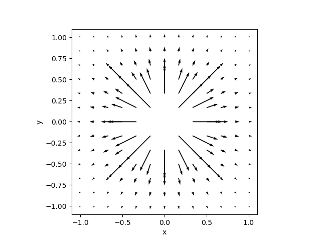
Returning to our original point charge, for the electric field from a positive point charge \(q\) acting on a positive test charge, we select signs and directions so that the force on the test charge will repel it in the positive \(\hat{r}\) direction: \[\vec{E} = \dfrac{k q}{r^2} \hat{r},\qquad{(1)}\] or equivalently, \[\vec{E} = \dfrac{1}{4\pi \epsilon_0} \dfrac{q}{r^2} \hat{r}.\qquad{(2)}\]

fig. 2 shows a visualization of an electric field for a point charge.

Figure 2: Notional inverse square law electric field for a positive point charge at (0,0). Large vectors near zero have been masked from the quiver plot. — Figure 2: Notional inverse square law electric field for a positive point charge at \((0,0)\). Large vectors near zero have been masked from the quiver plot.

Electric field from systems of point charges using superposition

As we did with electrostatic force, we can use (linear) superpositionfancy way to say we add things up

to find the resulting electric field from systems of point charges, or for distributions of charge densities by integrating \(\lambda\), \(\sigma\), or \(\rho\) over lines, areas, or volumes. For these latter cases, there may be easier methods, as we shall see later.

fig. 3, fig. 4 show visualizations of an electric field for two equal point charges near each other separated by a short distance.

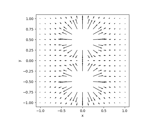
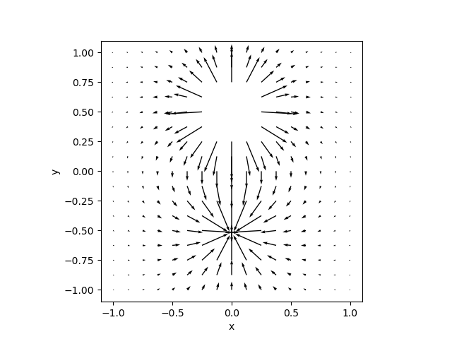
Figure 3: Electric field for two equal positive point charges separated by a short distance. Charges are at y=\pm 0.5 — Figure 3: Electric field for two equal positive point charges separated by a short distance. Charges are at \(y=\pm 0.5\)

Figure 4: Electric field for equal positive and negative point charges separated by a short distance, i.e. a dipole. Charges are at y=\pm 0.5 — Figure 4: Electric field for equal positive and negative point charges separated by a short distance, i.e. a dipole. Charges are at \(y=\pm 0.5\)

fig. 4 shows two equal but opposite point charges separated by a short distance. Field lines originate on the positive charge and end on the negative charge. Two equal and opposite charges separated a short distance in this way are called a dipole.

Navigation links

References

Pelcovits, Robert A, and Joshua Farkas. 2024. Barron’s AP Physics c Premium. Kaplan North America.

Tipler, Paul A, and Gene Mosca. 2004. Physics for Scientists and Engineers. 5th ed. W H Freeman; Company.