Electric potential for distributed charge configurations
Read Tipler and Mosca (2004) chapter 23 (Electric
potential); Pelcovits and
Farkas (2024) chapter 10 (Electrostatic) pp.289–302. See also https://en.wikipedia.org/wiki/Electric_potential
You ought to try these yourself.
Point charge and things that look like point charges
The magnitude of the electric field for a point charge is given by \[\begin{equation} E = \dfrac{k q}{r^2}. \end{equation}\]
Evaluating \(-\int \vec{E}\cdot d\vec{s}\) directly gives \[\begin{align} V &= -\int_\infty^r \dfrac{k q}{s^2} ds \\ &= \dfrac{k q}{r}. \end{align}\]
Charged ring with density \(\lambda\), C m−1
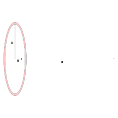
To find the potential for this configuration, we will integrate the charge around the ring: \[\begin{align} dV &= \dfrac{k dq}{r} \\ V &= \int \dfrac{k dq}{r} \\ &= \int_0^{2\pi} \dfrac{k \lambda R d\theta}{\sqrt{R^2+x^2}}. \label{eq:chargedring} \end{align}\] What is nice about this is that nearly all the terms in \[eq:chargedring\] pull out of the integral so that \[\begin{align} V &= \dfrac{k \lambda R}{\sqrt{R^2+x^2}} \int_0^{2\pi} d\theta \\ &= \dfrac{2 \pi k \lambda R}{\sqrt{R^2+x^2}} \\ &= \dfrac{k Q}{\sqrt{R^2+x^2}} = \dfrac{1}{4\pi\epsilon_0} \dfrac{Q}{\sqrt{R^2+x^2}} \end{align}\] where \(Q=2\pi R \lambda\) is the total charge on the ring.
Thin spherical shell with density \(\sigma\)
Recall that the electric field for a spherical shell can be obtained using Gauss’ law and is given by: \[\begin{equation} \vec{E}(r) = \begin{cases} 0 & r < R \\ \dfrac{4 \pi R^2 \sigma k}{r^2}\hat{r} & r \geq R \end{cases} \end{equation}\]
Let \(Q=4\pi R^2 \sigma\). We can then write the potential by inspection. Outside the sphere, the system looks like a point charge \(Q\). Inside the sphere, the electric field is zero and the electric potential is simply constant at a value chosen so that \(V\) inside and out match at \(r=R\): \[\begin{equation} V = \begin{cases} \dfrac{k Q}{R} & r < R \\ \dfrac{ k Q}{r} & r \geq R \end{cases} \end{equation}\]
Things that look like lines
Infinite wire with density \(\lambda\), C m−1
Recall the Gauss’s law solution for the electric field for an infinite line charge with charge density \(\lambda\) was: \[\begin{equation} \vec{E}(r) = 2 k \lambda \dfrac{1}{r} \hat{r}=\dfrac{\lambda}{2\pi\epsilon_0}\dfrac{1}{r}\hat{r}. \end{equation}\]
We can get the potential by evaluating \(-\int \vec{E}\cdot d\vec{s}\) directly, with one small wrinkle: \[\begin{align} V &= -\int_{r_0}^r \dfrac{2 k \lambda}{s} ds \\ &= \left. - 2 k \lambda \right|_{r_0}^r \\ &= -2 k \lambda \ln{\dfrac{r}{r_0}} = -\dfrac{\lambda}{2\pi\epsilon_0} \ln{\dfrac{r}{r_0}}. \end{align}\] Unlike in the solution for a point charge, we cannot take this integral out to \(r=\infty\) as the natural log will blow up. In practice, we instead pick some far distance \(r_0\) to that we call ground (\(V=0\)).
Infinite cylindrical shell with density \(\sigma\)
We will work this as we did for the spherical shell. Recall for a cylindrical shell, the electric field can be obtained from Gauss’ law and is given by \[\begin{equation} \vec{E}(r) = \begin{cases} 0 & r < R \\ 4\pi k \sigma R \dfrac{1}{r} \hat{r} = \dfrac{\sigma R}{\epsilon_0} \dfrac{1}{r} \hat{r} & r \geq R \end{cases} \end{equation}\]
Select \(\lambda = 2\pi R \sigma\) as the charge per unit length of the cylindrical shell. Outside the cylinder (\(r>R\)), it looks like out solution for the infinite wire. Inside the wire, the electric field is zero so the potential is constant, selected so that the potential inside and outside the cylinder match at \(r=R\). \[\begin{equation} V = \begin{cases} -2 k \lambda \ln{\dfrac{R}{r_0}} & r < R \\ -2 k \lambda \ln{\dfrac{r}{r_0}} & r \geq R. \end{cases} \end{equation}\] It is probably important to note that \(R \neq r_0\). \(R\) is the radius of the cylindrical shell; while \(r_0\) was some far off radius chosen to be our ground where \(V=0\).
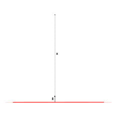
Infinite surface with density \(\sigma\), C m−2
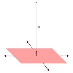
We used Gauss’s law to find the electric field for a plane: \[\begin{equation} \vec{E}(z) = \begin{cases} 2\pi k \sigma \hat{z} = \dfrac{\sigma}{2\epsilon_0} \hat{z} & z \geq 0 \\ -2\pi k \sigma \hat{z} = -\dfrac{\sigma}{2\epsilon_0} \hat{z} & z<0 \end{cases} \end{equation}\]
Doing the integral \(-\int \vec{E}\cdot d\vec{s}\) directly gives \[\begin{equation} V(z) = \begin{cases} -2\pi k \sigma z = - \dfrac{\sigma}{2\epsilon_0} z & z \geq 0 \\ 2\pi k \sigma z = \dfrac{\sigma}{2\epsilon_0} z & z<0. \end{cases} \end{equation}\]
Volumes
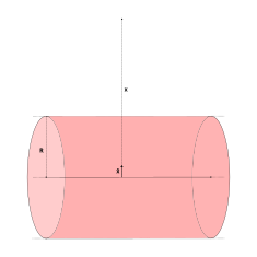
Infinite cylindrical volume with density \(\rho\), C m−3
The electric field from Gauss’ law is \[\begin{equation} \vec{E}(r) = \begin{cases} 2\pi k \rho r \hat{r} & r < R \\ 2\pi k \rho R^2 \dfrac{1}{r} \hat{r} & r \geq R, \end{cases} \end{equation}\] and the situation looks similar to the infinite wire and infinite cylindrical shell, except with the field growing linearly inside \(r<R\).
Integration gives \[\begin{equation} V(r) = \begin{cases} - 2\pi k \rho r^2 + C & r < R \\ - 2\pi k \rho R^2 \ln{\dfrac{r}{r_0}} \hat{r} & r \geq R, \end{cases} \end{equation}\] choosing \(C = 2\pi k \rho R^2 - 2\pi k \rho R^2 \ln{\dfrac{R}{r_0}}\) in order to have the potential match at \(r=R\).
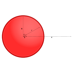
Spherical volume with density \(\rho\)
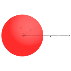
The electric field from Gauss’s law is \[\begin{equation} \vec{E}(r) = \begin{cases} \dfrac{4 \pi \rho k}{3} r \hat{r} & r < R \\ \dfrac{4 \pi R^3 \rho k}{3 r^2}\hat{r} & r \geq R \end{cases} \end{equation}\] and the situation looks similar to the point charge and spherical shell, except with the field growing linearly inside \(r<R\). Outside the sphere (\(r>R\)), the situation looks like a point charge of magnitude \(Q=\dfrac{4}{3}\pi R^3 \rho\).
Integration gives \[\begin{equation} V(r) = \begin{cases} -\dfrac{4\pi \rho k}{3} \dfrac{1}{2} r^2 + C & r < R \\ \dfrac{4 \pi R^3 \rho k}{3} \dfrac{1}{r} & r \geq R, \end{cases} \end{equation}\] choosing \(C = \dfrac{4\pi \rho k}{3} \dfrac{1}{2} R^2 + \frac{4}{3} \pi R^2 \rho k \dfrac{1}{R}\) so that the potential inside and outside match at \(r=R\).
If we pick \(Q=\dfrac{4}{3}\pi r^3 \rho\), and \(k=\dfrac{1}{4\pi\epsilon_0}\) these should simplify to \[\begin{equation} V(r) = \begin{cases} \dfrac{Q(3R^2-r^2)}{8\pi\epsilon_0 R^2} & r < R \\ \dfrac{Q}{4\pi\epsilon_0 r} & r \geq R. \end{cases} \end{equation}\]
Charged disk with density \(\sigma\)
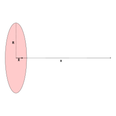
It is left to the student to show that \[\begin{equation} V = \dfrac{\sigma}{2\epsilon_0} \left[ \sqrt{x^2+R^2} - x \right] \end{equation}\] on the axis.
Electric dipole
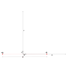
It is left to the student to show that \[\begin{equation} V(x) = \begin{cases} 0 & x=0\,\text{on the equitorial plane} \\ \dfrac{p}{4\pi\epsilon_0 x^2} & x >> d \end{cases} \end{equation}\] where \(p\) is the magnitude of electric dipole moment.
See also
- list here