Gauss’ law for electrostatics
Read Tipler and Mosca (2004) chapter 23 (Electric
potential); Pelcovits and
Farkas (2024) chapter 10 (Electrostatic) pp.289-302.
You should be able to describe the electric potential due
to a configuration of charged objects.
Electric potential
Electric potential describes the electric potential energy per unit charge at a point in space. \[\begin{equation} V = \dfrac{U_E}{q}. \end{equation}\]
Electric potential is a scalar, and is given the symbol \(V\) in AP Physics C material and is
measured in volts\(\qty{1}{\volt}=\qty{1}{\joule\per\coulomb}\).
Named for Count Alessandro Volta, Italian physicist and chemist credited
as inventor of the battery (inspired by the bio work of Luigi Galvani)
and discoverer of methane. See https://en.wikipedia.org/wiki/Alessandro_Volta.
(V). You may also see voltage given the symbol \(E\), \(\cal{E}\), or \(v\) (especially in context of electronics
or electrical engineering), or \(\phi\).
Electric potential for a point charge
We previously obtained the electric potential energy of a system of two point charges from the work needed to move the charges from being infinitely far away and assemble them into a configuration \(r\) distance apart: \[\begin{equation} U_E = \dfrac{1}{4\pi\epsilon_0}\dfrac{q_1 q_2}{r} = \dfrac{k q_1 q_2}{r}. \end{equation}\]
If we divide by the test charge, we obtain an expression for the electric potential of a single point charge, \(q\): \[\begin{equation} V = \dfrac{q}{4\pi\epsilon_0 r} \end{equation}\] where \(\epsilon_0\) is the permittivity of free space and \(r\) is the distance from the charge. When written in this way, the electric potential represents the work per (test) charge it would take to move a test charge from infinitely far away to a distance \(r\) from the original charge.
The electric potential difference between two points is the
change in electric potential energy per unit charge when a test charge
is moved between the two pointsEquation 11 on the official
AP Physics C Electricity & Magentism equation sheet
: \[\begin{equation}
\Delta V = \dfrac{\Delta U_E}{q}.
\end{equation}\]
Electric potential difference can result from chemical processes that cause positive and negative charges to separate, such as in a battery, due to corrosion of a metal, or as the result of biological pumping of ions; or it can occur from physical processes like the transfer of charges, photoelectric effects, physical stripping of electrons, etc.
Superposition applies!
The electric potential due to multiple point charges can be
determined using scalar superpositionEquation 8 on the official
AP Physics C Electricity & Magnetism equation sheet
of the electric potential due to each of the
point charges, e.g. for a collection of \(i\) charges, \[\begin{equation}
V = \dfrac{1}{4\pi\epsilon_0} \Sigma_i \dfrac{q_i}{r_i}
\end{equation}\]
Similarly, expressions for the electric potential of charge distributions can be found using integration and the principle of superposition: \[\begin{equation} V = \dfrac{1}{4\pi\epsilon_0} \int \dfrac{dq}{r}. \end{equation}\] This form is useful when you have some distribution of charge per unit length (\(\lambda, \unit{\coulomb\per\meter}\)), charge per unit area (\(\sigma, \unit{\coulomb\per\meter\squared}\)), or charge per unit volume (\(\rho, \unit{\coulomb\per\meter\cubed}\))
AP Physics C Electricity & Magnetism only expects
students to use calculus to find the electric potential resulting from
the following charge distributions and locations: an infinitely long,
uniformly charged wire or cylinder at a distance from its central axis;
a thin ring of charge at a location along the axis of the ring; a
semicircular arc or part of a semicircular arc at its center; and a
finite wire or line charge at a point collinear with the line charge or
at a location along its perpendicular bisector.
Relationships between electric potential and electric field
There are some key relationships between electric potential and electric field. Recall the electric field represents the force per unit charge felt by a test charge; it’s “like force”. Electric potential is the energy per unit charge; it’s “like energy”, and energy and work are related to force as the integral, i.e. \(W = \int F\cdot ds\).
Thus, electric potential is like the integral of electric field.
The change in electric potential between two points can be
determined by integrating the dot product of the electric field and the
displacement along the path connecting the pointsEquation 9 on the official
AP Physics C Electricity & Magnetism equation sheet
: \[\begin{equation}
\Delta V = V_b - V_a = - \int_a^b \mathbf{E} \cdot d\mathbf{r}.
\end{equation}\qquad{(1)}\]
The dot product enters here because work \(dW = \textbf{F}\cdot d\textbf{s}\). Electrostatic forces are conservative, so this integral should not depend on the actual path taken, only on the endpoints \(a\) and \(b\).
At this point, you have taken enough calculus that you know that when
we take an integral of a function, the inverse operation is sort of like
the derivative. Is there a way we can go from a known potential to an
electric field? Yes, sort of. In one dimensionEquation 10 on the official
AP Physics C Electricity & Magnetism equation sheet
: \[\begin{equation}
E_x = -\dfrac{dV}{dx}.
\end{equation}\qquad{(2)}\]
We have to be careful here because in eq. 1 we took a dot product. In general, the value of an electric field component in any direction at a given location is equal to the negative of the spatial rate of change in electric potential at that location.
Relationships between \(\vec{E}\) and \(\phi\) (\(\phi=V\)) in 3D (optional)
Not testable on the AP Physics C Electricity &
Magnetism exam but really useful.
More generally, we might write the potential as a scalar function of multiple variables, \(\phi=\phi(x,y,z)\). In multiple dimensions, eq. 2 is written as \[\begin{equation} \vec{E} = - \vec{\nabla} \phi \end{equation}\] where the \(\vec{\nabla}\) symbol is spoken as “del” and is given by \(\vec{\nabla}=\frac{\partial}{\partial x}\hat{i}+\frac{\partial}{\partial y}\hat{j}+\frac{\partial}{\partial z}\hat{k}\) in Cartesian coordinates. It is a vector operator, and in this case results in the gradient of the potential (also sometimes written as \(\text{grad} \phi\). This means that electric field lines point down the gradient of potential.
Going the other way, from electric field to potential, is still the same: \[\begin{equation} \phi = - \int \vec{E} \cdot d\vec{s}. \end{equation}\] but in this case we can see the dot product in action as the path we take may or may not be parallel to the electric field.
There’s one other really cool use of this. Recall Gauss’s Law, which we know as \(\oint \vec{E}\cdot d\vec{a} = 4\pi k q_{enc}\), in differential form is: \[\begin{equation} \vec{\nabla}\cdot \vec{E} = 4\pi k\rho = \dfrac{\rho}{\epsilon_0}, \end{equation}\] in other words, the divergence of the electric field (\(\text{div} \vec{E}\)) is proportional to the volumetric charge density \(\rho\).
Since we are also writing \(\vec{E}=-\vec{\nabla}\phi\), \[\begin{equation} \vec{\nabla}\cdot \vec{\nabla}\phi = \nabla^2\phi = -4\pi k\rho = -\dfrac{\rho}{\epsilon_0}, \end{equation}\qquad{(3)}\]
which is an example of Poisson’s Equation and has a catalog of nifty solutions. In regions where there is no charge, \(\rho=0\), and eq. 3 becomes \[\begin{equation} \nabla^2\phi = 0, \end{equation}\qquad{(4)}\] which is an example of Laplace’s Equation and has even easier-to-use solutions, and easy-to-use numerical solution methods, where you utilize the boundary conditions to pin down your solutions, often as superposition of solutions that are orthogonal functions. Such methods occur widely in electrostatics, also in gravitation, heat and mass transfer, fluid mechanics, nuclear reactor theory, diffusion, etc.
Visualizing electric field and electric potential
Electric field vector maps and equipotential lines (fig. 1) are tools to describe the field produced by a charge or a configuration of charges and can be used to predict the motion of charge objects in the field.
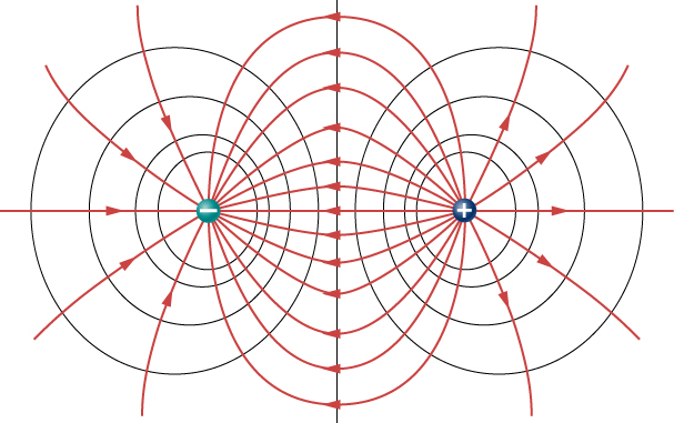
Equipotential lines represent lines of equal electric potential. These lines are also referred to as isolines of electric potential.
Equipotentials (isolines) are perpendicular to electric field vectors. An equipotential (isoline) map of electric potential can be constructed from an electric field vector map, and an electric field map may be constructed from an equipotential (isoline) map.
An electric field vector points in the direction of
decreasing potentialWhen we discussed diffusion in biology class we had a
similar idea; that diffusion acts with solutes moving down a
concentration gradient, \(\vec{J} = -D
\vec{\nabla} C\) for those freshmen who were good with vector
calculus and partial differential equations. The same thing happens
here; which you can also remember as the little electric field skier
dude going down the electric potential slope…
.
There is no component of an electric field along an equipotential
(isoline)Corollary to this is the electric field lines are
perpendicular to equipotentials.
.
See also
- list here